Automatic Control Knowledge Repository
You currently have javascript disabled. Some features will be unavailable. Please consider enabling javascript.Details for: "distillation column"
Name: distillation column
(Key: JBTRZ)
Path: ackrep_data/system_models/distillation_column_system View on GitHub
Type: system_model
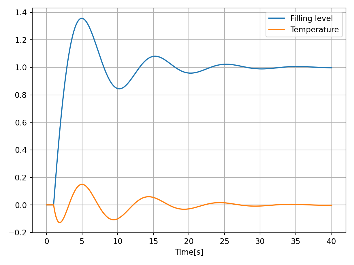
Short Description: conrol the filling level and temperature of the ground of the distillation column by the supply of the heat steam and the drain of the product
Created: 2022-09-12
Compatible Environment: default_conda_environment (Key: CDAMA)
Source Code [ / ] system_model.py
Related Problems:
Extensive Material:
Download pdf
Result: Success.
Last Build: Checkout CI Build
Runtime: 3.3 (estimated: 10s)
Plot:
The image of the latest CI job is not available. This is a fallback image.
Path: ackrep_data/system_models/distillation_column_system View on GitHub
Type: system_model
Short Description: conrol the filling level and temperature of the ground of the distillation column by the supply of the heat steam and the drain of the product
Created: 2022-09-12
Compatible Environment: default_conda_environment (Key: CDAMA)
Source Code [ / ] system_model.py
import sympy as sp
import symbtools as st
import importlib
import sys, os
import numpy as np
from pyblocksim import *

# from ipydex import IPS, activate_ips_on_exception

from ackrep_core.system_model_management import GenericModel, import_parameters

# Import parameter_file
params = import_parameters()


# link to documentation with examples: https://ackrep-doc.readthedocs.io/en/latest/devdoc/contributing_data.html


class Model(GenericModel):
    def initialize(self):
        """
        this function is called by the constructor of GenericModel

        :return: None
        """

        # ---------start of edit section--------------------------------------
        # Define number of inputs -- MODEL DEPENDENT
        self.u_dim = 7

        # Set "sys_dim" to constant value, if system dimension is constant
        self.sys_dim = 2

        # ---------end of edit section----------------------------------------

        # check existence of params file
        self.has_params = True
        self.params = params

    # ----------- SET DEFAULT INPUT FUNCTION ---------- #
    # --------------- Only for non-autonomous Systems
    def uu_default_func(self):
        """
        define input function

        :return:(function with 2 args - t, xx_nv) default input function
        """

        # ---------start of edit section--------------------------------------
        def uu_rhs(t, xx_nv):
            """
            sequence of numerical input values

            :param t:(scalar or vector) time
            :param xx_nv:(vector or array of vectors) numeric state vector
            :return:(list) numeric inputs
            """
            u1 = 1
            u2 = 1
            u3 = 1
            u4 = 1
            u5 = 1
            u6 = 1
            u7 = 1
            return [u1, u2, u3, u4, u5, u6, u7]

        # ---------end of edit section----------------------------------------

        return uu_rhs

    def get_rhs_func(self):
        msg = "This DAE model has no rhs func like ODE models."
        raise NotImplementedError(msg)

    def get_rhs_symbolic(self):
        """This model is not represented by the standard rhs equations."""
        return False

    def get_Blockfnc(self):
        """
        generate blockfunctions

        :return: (list) two blockfunctions and input
        """

        x1, x2 = self.xx_symb  # state components
        KR1, TN1, KR2, TN2, T1, K1, K2, K3, K4 = self.pp_symb  # parameters
        KR1 = self.pp_dict[KR1]
        TN1 = self.pp_dict[TN1]
        KR2 = self.pp_dict[KR2]
        TN2 = self.pp_dict[TN2]
        T1 = self.pp_dict[T1]
        K1 = self.pp_dict[K1]
        K2 = self.pp_dict[K2]
        K3 = self.pp_dict[K3]
        K4 = self.pp_dict[K4]

        # u1, u2, u3, u4, u5, u6, u7 = self.uu_symb   # inputs
        u1, u2, u3, u4, u5, u6, u7 = inputs("u1, u2, u3, u4, u5, u6, u7")

        DIF1 = Blockfnc(u3 - u1)
        DIF2 = Blockfnc(-u2)

        PI1 = TFBlock(KR1 * (1 + 1 / (s * TN1)), DIF1.Y)
        PI2 = TFBlock(KR2 * (1 + 1 / (s * TN2)), DIF2.Y)

        SUM11 = Blockfnc(PI1.Y + u4)
        SUM21 = Blockfnc(PI1.Y + u5)

        SUM12 = Blockfnc(PI2.Y + u6)
        SUM22 = Blockfnc(PI2.Y + u7)

        P11 = TFBlock(K1 / s, SUM11.Y)
        P21 = TFBlock(K4 / (1 + s * T1), SUM21.Y)
        P12 = TFBlock(K3 / s, SUM12.Y)
        P22 = TFBlock(K2 / s, SUM22.Y)

        SUM1 = Blockfnc(P11.Y + P12.Y)
        SUM2 = Blockfnc(P22.Y + P21.Y)

        loop(SUM1.Y, u1)
        loop(SUM2.Y, u2)

        return [SUM1, SUM2, u3]
import numpy as np
import system_model
from scipy.integrate import solve_ivp
from pyblocksim import *

from ackrep_core import ResultContainer
from ackrep_core.system_model_management import save_plot_in_dir
import matplotlib.pyplot as plt
import os

# link to documentation with examples: https://ackrep-doc.readthedocs.io/en/latest/devdoc/contributing_data.html


def simulate():
    """
    simulate the system model

    :return: simulation data
    """

    model = system_model.Model()

    # rhs_xx_pp_symb = model.get_rhs_symbolic()
    # print("Computational Equations:\n")
    # for i, eq in enumerate(rhs_xx_pp_symb):
    #     print(f"dot_x{i+1} =", eq)

    # ---------start of edit section--------------------------------------

    SUM1, SUM2, u3 = model.get_Blockfnc()

    thestep = stepfnc(1.0, 1)

    t, states = blocksimulation(40, (u3, thestep), dt=0.05)

    bo = compute_block_ouptputs(states)

    simulation_data = [t, bo[SUM1], bo[SUM2]]

    # ---------end of edit section----------------------------------------

    save_plot(simulation_data)

    return simulation_data


def save_plot(simulation_data):
    """
    plot data and save the plot

    :param simulation_data: simulation_data of system_model
    :return: None
    """
    # ---------start of edit section--------------------------------------
    # plot of your data
    plt.plot(simulation_data[0], simulation_data[1], label="Filling level")
    plt.plot(simulation_data[0], simulation_data[2], label="Temperature")
    plt.xlabel("Time [s]")
    plt.legend()
    plt.grid()
    # ---------end of edit section----------------------------------------

    plt.tight_layout()

    save_plot_in_dir()


def evaluate_simulation(simulation_data):
    """
    assert that the simulation results are as expected

    :param simulation_data: simulation_data of system_model
    :return:
    """
    # ---------start of edit section--------------------------------------
    # fill in final states of simulation to check your model
    # simulation_data.y[i][-1]
    expected_final_state = [40.05, 0.99676226, -2.16627258e-03]

    # ---------end of edit section----------------------------------------

    rc = ResultContainer(score=1.0)
    simulated_final_state = [simulation_data[0][-1], simulation_data[1][-1], simulation_data[2][-1]]
    rc.final_state_errors = [
        simulated_final_state[i] - expected_final_state[i] for i in np.arange(0, len(simulated_final_state))
    ]
    rc.success = np.allclose(expected_final_state, simulated_final_state, rtol=0, atol=1e-2)

    return rc
import sys
import os
import numpy as np
import sympy as sp

import tabulate as tab


# link to documentation with examples: https://ackrep-doc.readthedocs.io/en/latest/devdoc/contributing_data.html


# set model name
model_name = "distillation column"


# ---------- create symbolic parameters
pp_symb = [KR1, TN1, KR2, TN2, T1, K1, K2, K3, K4] = sp.symbols("KR1, TN1, KR2, TN2, T1, K1, K2, K3, K4", real=True)


# ---------- create symbolic parameter functions
# parameter values can be constant/fixed values OR set in relation to other parameters (for example: a = 2*b)
KR1_sf = 1.7
TN1_sf = 1.29

KR2_sf = 0.57
TN2_sf = 1.29

### Plant
T1_sf = 1.0

# equilibrium pojnt 1
K1_sf, K2_sf, K3_sf, K4_sf = 0.4, 1.2, -0.8, -0.2

# equilibrium point 2
# K1_sf, K2_sf, K3_sf, K4_sf = 0.4, 1.2, -1.28, -0.32

# switch of coupling:
# K3_sf, K4_sf = 0,0


# list of symbolic parameter functions
# tailing "_sf" stands for "symbolic parameter function"
pp_sf = [KR1_sf, TN1_sf, KR2_sf, TN2_sf, T1_sf, K1_sf, K2_sf, K3_sf, K4_sf]


#  ---------- list for substitution
# -- entries are tuples like: (independent symbolic parameter, numerical value)
pp_subs_list = []


# OPTONAL: Dictionary which defines how certain variables shall be written
# in the table - key: Symbolic Variable, Value: LaTeX Representation/Code
# useful for example for complex variables: {Z: r"\underline{Z}"}
latex_names = {KR1: r"K_{R1}", TN1: r"T_{N1}", KR2: r"K_{R2}", TN2: r"T_{N2}"}


# ---------- Define LaTeX table

# Define table header
# DON'T CHANGE FOLLOWING ENTRIES: "Symbol", "Value"
tabular_header = ["Symbol", "Value"]

# Define column text alignments
col_alignment = ["center", "left"]


# Define Entries of all columns before the Symbol-Column
# --- Entries need to be latex code
col_1 = []

# contains all lists of the columns before the "Symbol" Column
# --- Empty list, if there are no columns before the "Symbol" Column
start_columns_list = []


# Define Entries of the columns after the Value-Column
# --- Entries need to be latex code
col_4 = []

# contains all lists of columns after the FIX ENTRIES
# --- Empty list, if there are no columns after the "Value" column
end_columns_list = []
Related Problems:
Extensive Material:
Download pdf
Result: Success.
Last Build: Checkout CI Build
Runtime: 3.3 (estimated: 10s)
Plot:
The image of the latest CI job is not available. This is a fallback image.